Bar Chart Race in Python with Matplotlib

04. Sep 2019

5 minutes read

~In roughly less than 50 lines of code

Bar chart races have been around for a while. This year, they took social media by storm. It began with Matt Navarra’s tweet, which was viewed 10 million times. Then, John Burn-Murdoch created reproducible notebook using d3.js, others started creating their races. Then, Flourish studio released race chart for non-programmers. Since then hundreds of races have been shared on the Internet.

Race with Matplotlib

I wondered – How easy would it be to re-produce JBM’s version in Python using Jupyter and Matplotlib? Turns out, in less than 50 lines of code, you can reasonably re-create reusable bar chart race in Python with Matplotlib.

Here’s what we want to create.

bar chart race

Let’s Code

Now, that you’ve seen the output, we’ll incrementally build it up.

Matplotlib's style defaults are designed for many common situations, but are in no way optimal for our aesthetics. So, bulk of our code would go into styling (axes, text, colors, ticks etc)

In your Jupyter notebook, import the dependent libraries.

import pandas as pd
import matplotlib.pyplot as plt
import matplotlib.ticker as ticker
import matplotlib.animation as animation
from IPython.display import HTML

Read the city populations dataset with pandas. We only need 4 columns to work with 'name', 'group', 'year', 'value'. Typically, a name is mapped to a group (city to continent/country) and each year has one value.

df = pd.read_csv('https://git.io/fjpo3', usecols=['name', 'group', 'year', 'value'])
df.head(3)

	name	group	year	value
0	Agra	India	1575	200.0
1	Agra	India	1576	212.0
2	Agra	India	1577	224.0

Data transformations

We are interested to see top 10 values are a given year. Using pandas transformations, we will get top 10 values.

current_year = 2018
dff = df[df['year'].eq(current_year)].sort_values(by='value', ascending=True).head(10)
dff

	name	group	year	value
6045	Tokyo	Asia	2018	38194.2
1324	Delhi	India	2018	27890.0
5547	Shanghai	Asia	2018	25778.6
689	Beijing	Asia	2018	22674.2
3748	Mumbai	India	2018	22120.0
5445	Sao Paulo	Latin America	2018	21697.8
3574	Mexico City	Latin America	2018	21520.4
4679	Osaka	Asia	2018	20409.0
1195	Cairo	Middle East	2018	19849.6
1336	Dhaka	Asia	2018	19632.6

Basic chart

Now, let’s plot a basic bar chart. We start by creating a figure and an axes. Then, we use ax.barh(x, y) to draw horizontal barchart.

fig, ax = plt.subplots(figsize=(15, 8))
ax.barh(dff['name'], dff['value'])

basic

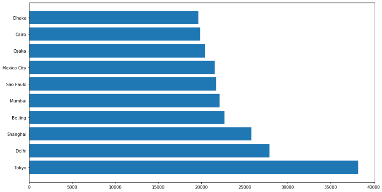
Notice, highest bar is at the bottom. We need to flip that.

Color, Labels

Next, let’s add values, group labels and colors based on groups. We’ll user colors and group_lk to add color to the bars.

colors = dict(zip(
    ['India','Europe','Asia','Latin America','Middle East','North America','Africa'],
    ['#adb0ff', '#ffb3ff', '#90d595', '#e48381', '#aafbff', '#f7bb5f', '#eafb50']
))
group_lk = df.set_index('name')['group'].to_dict()

group_lk is mapping between name and group values.

fig, ax = plt.subplots(figsize=(15, 8))
dff = dff[::-1]   # flip values from top to bottom

# pass colors values to `color=`

ax.barh(dff['name'], dff['value'], color=[colors[group_lk[x]] for x in dff['name']])
# iterate over the values to plot labels and values (Tokyo, Asia, 38194.2)

for i, (value, name) in enumerate(zip(dff['value'], dff['name'])):
    ax.text(value, i,     name,            ha='right')  # Tokyo: name

    ax.text(value, i-.25, group_lk[name],  ha='right')  # Asia: group name

    ax.text(value, i,     value,           ha='left')   # 38194.2: value

# Add year right middle portion of canvas

ax.text(1, 0.4, current_year, transform=ax.transAxes, size=46, ha='right')

labels

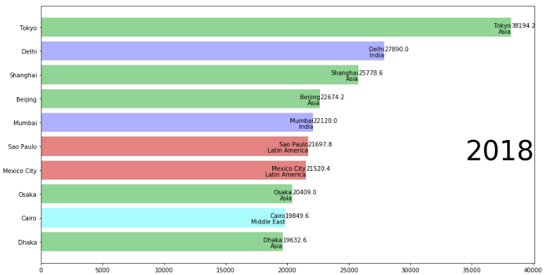
Now, we’re left with styling the chart.

Polish Style

For convenience let’s move our code to draw_barchart function.

We need to style following items:

Text: Update font sizes, color, orientation
Axis: Move X-axis to top, add color & subtitle
Grid: Add lines behind bars
Format: comma separated values and axes tickers
Add title, credits, gutter space
Remove: box frame, y-axis labels

We’ll add another dozen lines of code for this.

fig, ax = plt.subplots(figsize=(15, 8))

def draw_barchart(year):
    dff = df[df['year'].eq(year)].sort_values(by='value', ascending=True).tail(10)
    ax.clear()
    ax.barh(dff['name'], dff['value'], color=[colors[group_lk[x]] for x in dff['name']])
    dx = dff['value'].max() / 200
    for i, (value, name) in enumerate(zip(dff['value'], dff['name'])):
        ax.text(value-dx, i,     name,           size=14, weight=600, ha='right', va='bottom')
        ax.text(value-dx, i-.25, group_lk[name], size=10, color='#444444', ha='right', va='baseline')
        ax.text(value+dx, i,     f'{value:,.0f}',  size=14, ha='left',  va='center')
    # ... polished styles

    ax.text(1, 0.4, year, transform=ax.transAxes, color='#777777', size=46, ha='right', weight=800)
    ax.text(0, 1.06, 'Population (thousands)', transform=ax.transAxes, size=12, color='#777777')
    ax.xaxis.set_major_formatter(ticker.StrMethodFormatter('{x:,.0f}'))
    ax.xaxis.set_ticks_position('top')
    ax.tick_params(axis='x', colors='#777777', labelsize=12)
    ax.set_yticks([])
    ax.margins(0, 0.01)
    ax.grid(which='major', axis='x', linestyle='-')
    ax.set_axisbelow(True)
    ax.text(0, 1.12, 'The most populous cities in the world from 1500 to 2018',
            transform=ax.transAxes, size=24, weight=600, ha='left')
    ax.text(1, 0, 'by @pratapvardhan; credit @jburnmurdoch', transform=ax.transAxes, ha='right',
            color='#777777', bbox=dict(facecolor='white', alpha=0.8, edgecolor='white'))
    plt.box(False)
    
draw_barchart(2018)

2018full

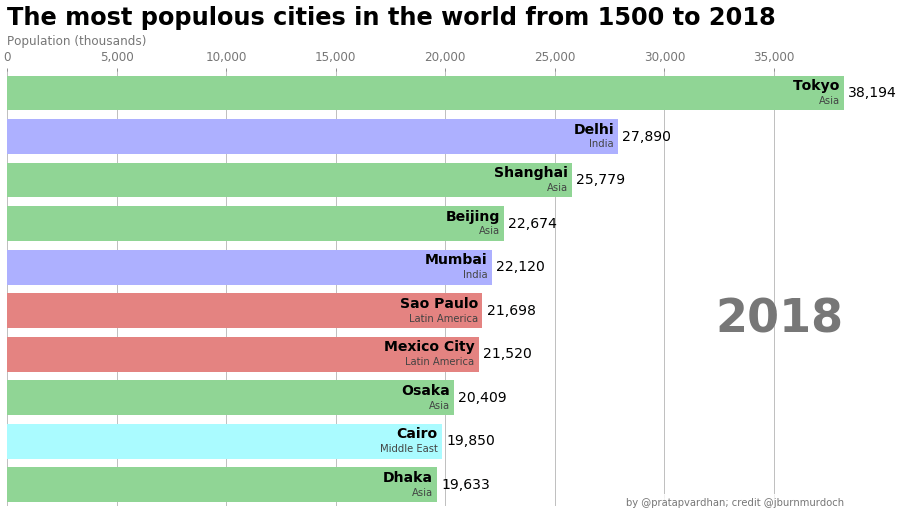
We now have an identical chart.

Animate Race

To animate the race, we will use FuncAnimation from matplotlib.animation. FuncAnimation makes an animation by repeatedly calling a function (that draws on canvas). In our case, that function will be draw_barchart. We also use frames, this argument accepts on what values you want to run draw_barchart – we’ll run from year 1968 to 2018.

import matplotlib.animation as animation
from IPython.display import HTML

fig, ax = plt.subplots(figsize=(15, 8))
animator = animation.FuncAnimation(fig, draw_barchart, frames=range(1968, 2019))
HTML(animator.to_jshtml()) 
# or use animator.to_html5_video() or animator.save()

And, there, we have it, bar chart race inside a notebook with matplotlib.

2018full

You could save the animator object to a video/gif or play within the notebook.

Bonus: xkcd-style!

Turning your matplotlib plots into xkcd styled ones is pretty easy. You can simply turn on xkcd sketch-style drawing mode with plt.xkcd.

with plt.xkcd():
    fig, ax = plt.subplots(figsize=(15, 8))
    draw_barchart(2018)

xkcd

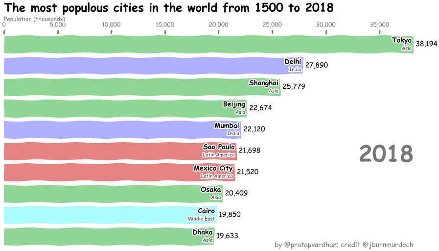
Here’s the animated xkcd-styled bar chart race.

DIY

Full code for the race animation is here and you can play with it on Google Colab also. Try changing the dataset, colors and share your races.

Matplotlib is a massive library – being able to adjust every aspect of a plot is powerful but it can be complex / time-consuming for highly customized charts. Atleast, for these bar chart races, it was fairly quick!

Tags / animation visualization python matplotlib

Pratap Vardhan